Demonstrating the Equivalence of a Global fit and an individual/merge fit of Gas Thermometric Data to find Absolute Zero
Carl Salter Moravian College
The global least squares fit has been published in the Journal of Chemical Education 2003, 80, pg 1033.
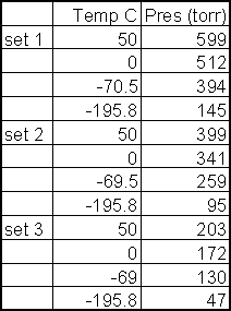
The data come from an experiment done by Moravian College physical chemistry students during the Fall 2000 semester. Three samples of helium gas were trapped in a steel sphere and subjected to four different temperatures. Pressures were measured using a digital pressure meter, least count 1 torr.
The Data

A global fit of the data forces all three lines to have a common x intercept.
This is accomplished easily in Excel using absolute cell references. (There
is a typegraphical error in the published version of the spreadsheet in JCE.
The fit function formula in column E should refer to column H, not column
I. The caption is correct; it refers to column H.)
The fit is performed using Solver; error propagation using SolverAid.
Results of the Global Fit
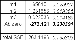
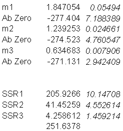
The Individual/Merge Fit Procedure should be equivalent. The procedure starts with fits of each set of data to a slope and an x intercept. These are nonlinear fits; they were also accomplished in Excel using Solver and SolverAid.
Results of the Individual Fits
The Merge Fit
For n data and p parameters the general equations for weighted least-squares are
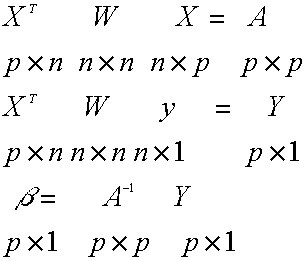
The X matrix is the matrix of derivatives of the fit function wrt to fit parameters, and contains the x data; the W matrix is the weight matrix. The A matrix is often called the model matrix. y is the vector of y data. b is the vector of parameters.
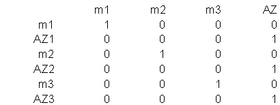
The merge fit is the fit of the parameters from the individual fits to the parameters of the global fit. The parameters from the individual fits are the "y data", so n=6, and p=4 since there will be three slopes and one value of absolute zero in the merge fit. The model equations are m1=m1, m2=m2, m3=m3, and AZ =AZ1 = AZ2 =AZ3. W is a block diagonal matrix containing the A matrices of the individual fits.
X matrix that results from the model equations
W matrix (A matrices from individual fits)

A matrix

A-1

y vector parameters from individual fits

Y vector

b (parameter) vector = A-1 Y

Error Propagation
The equations for error propagation are
![]()
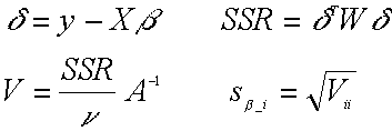
where delta is the residuals vector and SSR is the sum of the squared (weighted) residuals. V, the variance-covariance matrix, is computed by multiplying A-1 by the fit variance Sy2, which is SSR divided by the number of degrees of freedom of the fit, nu =n-p. The diagonal elements of V are the variances of the fit parameters.
For the individual/merge fit procedure, SSR must be the sum of the SSRs of the three individual fits plus the SSR from the merge fit. The resulting total SSR must equal the SSR of the global fit (a sort of conservation of squared residuals principle).
delta vector

SSR(merge) =11.73233
SSR(ind fit set 1) = 205.9266
SSR(ind fit set 2)= 41.4526
SSR(ind fit set 3) = 4.2586
SSR(total) =263.3702
Sy2 (ind/merge) = 32.92127
V matrix = Sy2 A-1

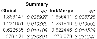
Note the excellent agreement of the two sets of fit parameters and their errors. The parameters obtained from the two procedures agree well within the stated standard deviations. In general the off-diagonal elements of the two V matrices agree to two significant digits.
An important point is that the global value of absolute zero is closest to the value obtained from the fit with the highest slope, set 1. This happens despite the fact that set 1 has the largest fit error. The weight matrix contains a higher weight for AZ1 (13.6) than for AZ2 (6.1) and AZ3 (1.6), which is why AZ is closest to AZ1. The weights are proportional to the square of the slope, so the AZ value associated with the highest slope receives the highest weight.
For more about using Solver and SolverAid in Excel to perform nonlinear fits, see the paper by me and Robert de Levie, J. Chem. Educ. 2002, vol 79, pg 268.
For more on global and merge fits, see the paper by Joel Tellinghuisen in J. Mol. Spec. 1996, vol 179, pg 299.